New R Package: transitreg for Flexible Transition Models

GitHub

transitreg is a new R package designed for probabilistic modeling of continuous and count data using transition models. Traditionally used in ordinal regression and count data modeling, transition models estimate probabilities of exceeding certain thresholds rather than assuming fixed parametric distributions. This makes them particularly useful for distributional regression, quantile regression, and full probabilistic modeling.

What Does transitreg Do?

• Extends transition models beyond count data to handle continuous responses.
• Uses a slicing technique to transform continuous data into a count-like representation, enabling estimation via binary regression methods.
• Supports distributional regression, allowing estimation of quantiles, full probability densities, and modal regression.
• Efficiently handles complex data structures, including excess zeros and non-standard distributions.
• Implements fast estimation algorithms, making it applicable to large-scale datasets.

How to Install transitreg

The package is currently available on GitHub, with a CRAN release planned for Summer 2025.

## Install the latest development version.
remotes::install_github("retostauffer/transitreg")

The main model fitting function is ?transitreg.

Why Use transitreg?

• More flexible than traditional distributional regression (no need for strict parametric assumptions).
• Handles excess zeros and complex distributions better than standard approaches.
• Computationally efficient – can be used on large datasets.
• Seamless integration with existing GAM-based software mgcv.

Example

Load the WeatherGermany data available on GitHub.

if(!("WeatherGermany" %in% installed.packages())) {
  remotes::install_github("gamlss-dev/WeatherGermany")
}
data(WeatherGermany, package = "WeatherGermany")
print(head(WeatherGermany))

  id       date Wmax pre Tmax Tmin sun name alt     lat    lon
1  1 1981-01-01   NA 1.7  3.4 -5.0  NA Aach 478 47.8413 8.8493
2  1 1981-01-02   NA 1.7  1.2 -0.4  NA Aach 478 47.8413 8.8493
3  1 1981-01-03   NA 5.4  5.4  1.0  NA Aach 478 47.8413 8.8493
4  1 1981-01-04   NA 8.8  5.6 -0.4  NA Aach 478 47.8413 8.8493
5  1 1981-01-05   NA 3.7  1.2 -2.4  NA Aach 478 47.8413 8.8493
6  1 1981-01-06   NA 4.0  1.2 -2.2  NA Aach 478 47.8413 8.8493

Subset for Falkenberg in Bavaria.

d <- subset(WeatherGermany, name == "Falkenberg,Kr.Rottal-Inn")

Visualize the distribution of daily precipitation observations.

hist(d$pre, freq = FALSE)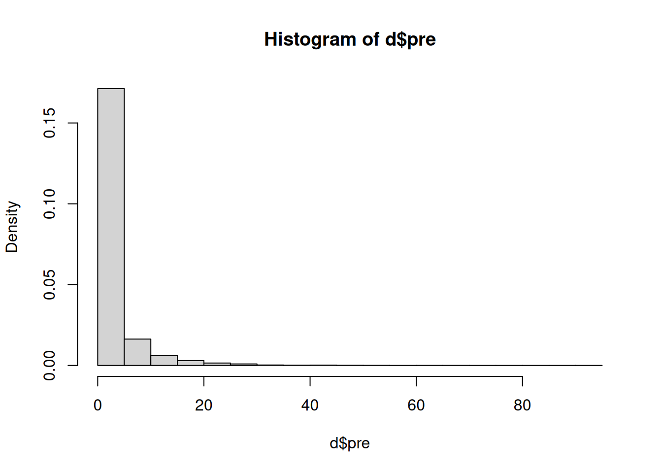

A square root tranformation is usually used for modeling.

d$sqrt_pre <- sqrt(d$pre)
hist(d$sqrt_pre, freq = FALSE)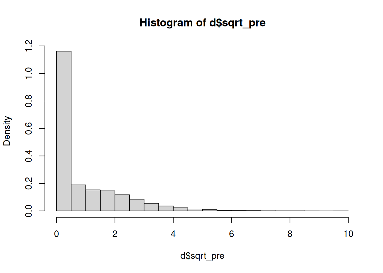

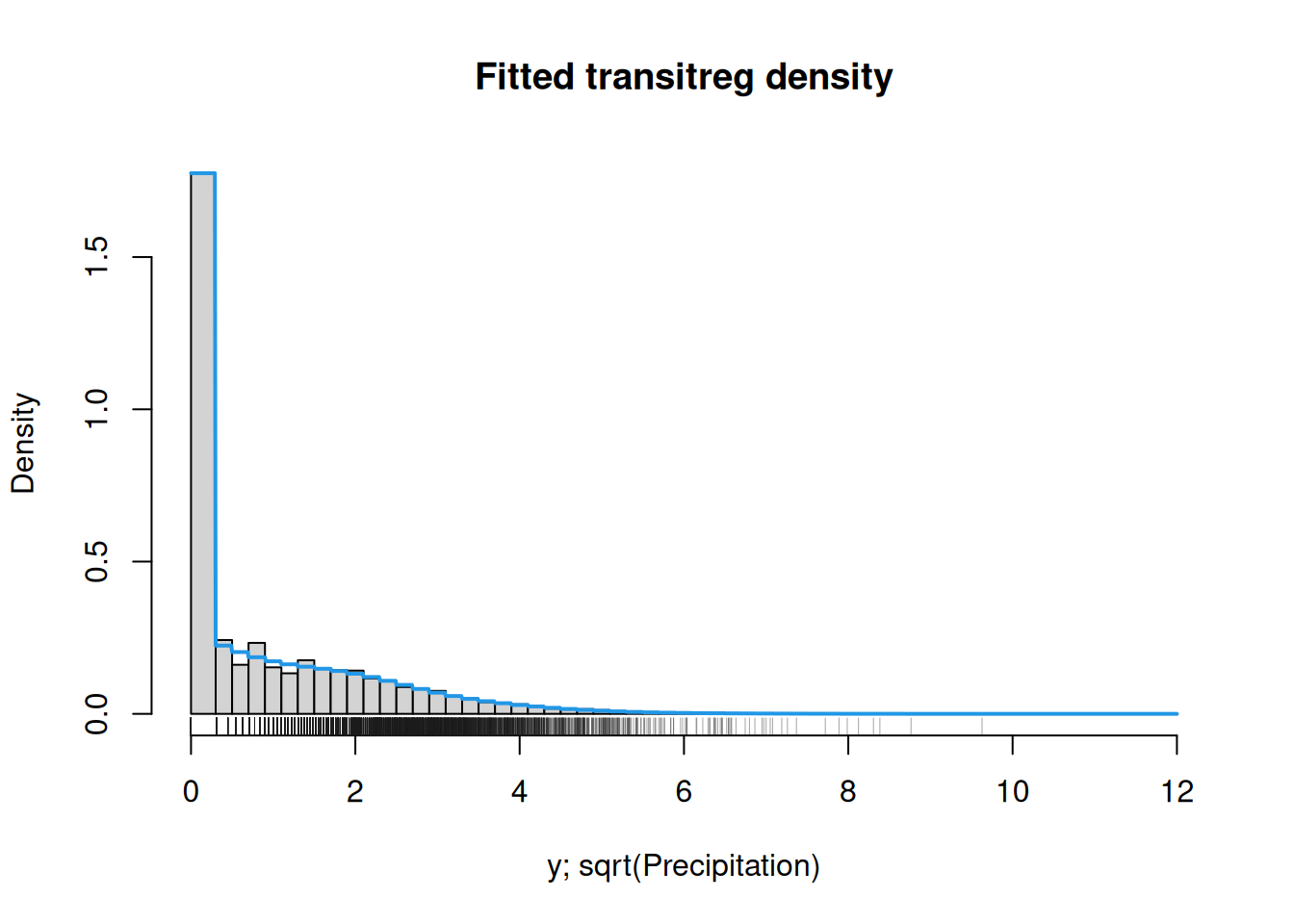
Fit a transition model that accounts for zero precipitation and visualize the fitted density.

library("transitreg")

## Set breaks, first break accounts for zero precipitation.
breaks <- c(0, seq(0.3, 12, by = 0.2))

## Estimate model.
b <- transitreg(sqrt_pre ~ theta0 + s(theta), data = d, breaks = breaks)

## Setup new data to predict the fitted density.
x <- c(0, 0.3, ((head(breaks, -1) + tail(breaks, -1L)) / 2)[-1])
nd <- data.frame("sqrt_pre" = x)
mids <- nd$sqrt_pre

## Predict.
py <- seq(0, 12, by = 0.01)
pm <- as.vector(predict(b, newdata = nd[1, , drop = FALSE], y = py, type = "pdf"))

## Visualize the precipitation distribution.
hist(d$sqrt_pre, breaks = breaks, freq = FALSE,
  xlab = "y; sqrt(Precipitation)", main = "Fitted transitreg density",
  xlim = c(0, 12))

## Add fitted density and rug plot of raw observations.
lines(pm ~ py, col = 4, lwd = 2)
rug(d$sqrt_pre, col = rgb(0.1, 0.1, 0.1, alpha = 0.4))